Keywords
INTRODUCTION
Effective prevention of sudden death presents substantial difficulties.1-4 Treatment of ventricular fibrillation (VF) is based on cardioversion by electrical shock, and implantable cardioverter defibrillators have proved useful in the prevention of death from arrhythmia.5-7 Other approaches exist for which the clinical results are yet to be revealed8-10 or which are not clinically applicable,11 and their further development requires an improved understanding of the physiologic basis and mechanisms that sustain arrhythmia.11-13 The techniques and methods used to study VF have had a notable influence on the analysis of such mechanisms. Both in the time and frequency domains, mapping techniques14-23 have allowed accurate information to be obtained that has been used to support various hypotheses regarding the onset, maintenance, and termination of this arrhythmia.11-14,22 One of the variables used is the activation frequency during VF, and analysis of both temporal and regional variations in this parameter has revealed inconsistent results.14-17,23-28 Spectral techniques have been widely used to obtain information on variability in activation frequency; however, one of the limitations of those techniques is the temporal resolution of the measurements, which is insufficient to allow determination of rapid or transient variations. The introduction of methods for time-frequency analysis has extended the opportunities for assessment of temporal variations and has opened the way for new approaches to the understanding of the mechanisms that sustain VF.21,28-31 In this study, we used time-frequency analysis in an experimental model of VF to analyze variations in frequency and spatial distribution over a short timescale.
METHODS
Experimental Preparation
The experimental procedures used were in accordance with current guidelines on the care and use of animals. Isolated perfused hearts were prepared from New Zealand rabbits (n=10; weight, 2.8±0.2 kg). Following anesthesia with intramuscular ketamine (25 mg/kg) and heparinization, the heart was removed and submerged in cold Tyrode's solution (4oC). Once the aorta was isolated, it was connected to a Langendorff system to perfuse Tyrode's solution at a pressure of 60 mm Hg and a temperature of 37±0.5°C. Oxygenation was performed with a mixture of 95% O2 and 5% CO2. Epicardial electrograms were recorded on the anterolateral wall of the left ventricle with a multiple electrode consisting of a plate with 240 unipolar electrodes (diameter, 0.125 mm; distance between electrodes, 1 mm). The reference electrode was a 4x6 mm Ag/AgCl plate placed on the aorta. Ventricular stimulation was performed using bipolar electrodes with a GRASS S88 stimulator coupled to an SIU5 stimulus isolator. Recordings were made using a mapping system for cardiac electrical activity (MAPTECH). Electrograms were amplified with a gain of 50 to 300 and were filtered over a frequency range of 1 to 400 Hz. Sampling was performed at a frequency of 1 kHz.
Experimental Protocol and Study Variables
Thirty minutes after placement of the electrodes, VF was induced by ventricular pacing at increasing frequencies (4 to 20 Hz) and VF recordings were obtained over 5-min periods; perfusion was maintained during the arrhythmia. The recordings analyzed corresponded to 2 segments of 4096 ms, separated by an interval of 2 s, obtained 5 minutes after the onset of the arrhythmia, a time point which corresponds to a stable phase in the VF in the type of experimental preparation used.18,20,32
Spectral Analysis of Ventricular Fibrillation
The method described by Welch33 was used to obtain the frequency spectrum of the signals recorded with each of the unipolar electrodes that make up the multiple electrode. The Fourier transform was calculated separately for each of the 2 segments of 4096 ms analyzed. Each segment was made up of 4096 points (sampling frequency, 1 kHz). Using the Welch method, the analysis was performed by taking the average of 3 segments, each with 2048 points and an overlap of 1024 points (firstly, the first 2048 points, secondly the points from 1024 to 3072, and thirdly, the points from 2048 to 4096). The analysis used a Hanning window, and to avoid the use of zero padding, 2n samples were taken. The dominant frequency (DF) for each electrode was obtained by determining the frequency with the greatest spectral power, with an effective spectral resolution of 0.5 Hz.
Time-Frequency Analysis of Ventricular Fibrillation
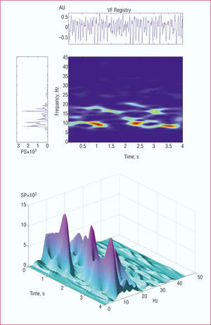
For time-frequency analysis21,28,29 (Figure 1), the signal corresponding to each segment was sampled at a frequency of 500 Hz. To obtain the spectrogram, a short Fourier transform was applied with a Hamming analysis window of 512 points. Determination of the spectrum of the analysis window was repeated iteratively, shifting it each time by 4 ms along the length of each 4096 ms segment. Zero padding was not used and the effective spectral resolution was 1 Hz. The following information was obtained:

Figure 1. The upper part of the figure shows the spectral and time-frequency analysis of the ventricular fibrillation signal. The spectrogram shown vertically corresponds to the entire segment analyzed with the Welch method. The time-frequency diagram shows the temporal change in the frequencies over the entire segment analyzed. A three-dimensional representation is shown in the lower part of the figure. VF indicates ventricular fibrillation; SP, spectral power; AU, arbitrary units.
- Temporal changes in the DF at each electrode over the 2 segments analyzed in each experiment
- Distribution of DF values in the area explored by construction of frequency maps and location of the maximum values in each of the 5 zones into which the analyzed area was divided (Figure 2)

Figure 2. Diagram of the epicardial multiple electrode situated on the anterolateral wall of the left ventricle, showing the 5 zones into which the area was divided. AD indicates anterior descending artery; RV(ant), anterior right ventricle; LV(ant), anterior left ventricle; LV(post), posterior left ventricle.
Statistical Analysis
Mean, SD, and coefficient of variation were calculated for the qualitative variables. Comparisons were made using a general linear model with a repeated measures test (SPSS statistical package). The within-individual variable was time and the between-individual variable was study zone. The Bonferroni test was used for post hoc analysis (multiple comparisons). A P value of less than .05 was considered statistically significant.
RESULTS
Temporal Variation in Dominant Frequency
Figure 3 shows the DF values obtained over a period of 4 s with 3 different electrodes in a single experiment. It can be seen that this parameter, obtained through time-frequency analysis, is not stable and that there are differences in the temporal patterns. The lower right hand graph shows the temporal change in the mean and SD of the DF values for all of the electrodes in the same experiment. It can be seen that the mean DF also varies according to the time elapsed, with a minimum of 14.5 Hz at 208 ms and a maximum value of 16.3 Hz at 1296 ms. The SD ranges from 1.9 to 3.3 Hz. Table 1 shows the means ± SD of the values for DF obtained with all of the electrodes at 4 different moments in time (500, 1500, 2500, and 3500 ms) over the 2 segments analyzed in each experiment. In all cases, with the exception of one case during the second segment of time analyzed, there were significant differences between some of the time points considered and the means of the coefficients of variation, which ranged from 0.19±0.06) to 0.22±0.07 (not significant). Linear regression analysis revealed a good correlation between the DF values obtained with the Welch method and those obtained with the time-frequency method (mean of all the measurements made at each specific time point): DF (Welch)=1.01xDF (time-frequency)0.4 (r=0.9; P<.0001; standard error of the estimate, 2.2 Hz). Comparison of the mean DF values obtained with the Welch method separately in the first and second segment revealed no significant differences; the values obtained were practically identical. Comparison of the means of all the DF values obtained with the time-frequency method in the first and second segment revealed statistically significant differences in 4 experiments.

Figure 3. Temporal changes in the DF value over a period of 4 s corresponding to recordings at 3 different electrodes in the same experiment. The lower right hand graph shows the temporal change in the mean and SD of the DF for all of the electrodes in the same experiment.

Spatial Variation in Dominant Frequency
Distribution of Dominant Frequency Values in the Area Analyzed
Table 2 shows the means (SD) for the DF values corresponding to all recordings in each of the 5 zones over the 2 time segments analyzed in each experiment. The differences between the zones were statistically significant in all cases. During the first time segment, the highest values were obtained in the apical and anterior zones, with the exception of 1 experiment in which those values were obtained in the posterior zone. In the second segment, the apical and anterior zone also corresponded to the highest mean values, except in 2 experiments where those values were obtained in the posterior zone.

Localization of Maximum Dominant Frequency Values
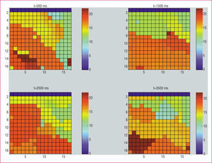
Figure 4 shows the frequency maps obtained in one of the experiments at 4 different time points in the same segment (500, 1500, 2500, and 3500 ms). These maps reveal temporal differences in the location of the maximum values. Table 3 shows the number of times that the maximum DF value was observed in each of the 5 zones, considering data obtained at 500, 1500, 2500, and 3500 ms with the time-frequency method. The maximum value was detected most frequently in the anterior and apical zones. Table 3 also shows the number of times that the maximum DF value was observed in each of the 5 zones for data obtained with the Welch method in each of the time segments. Using the Welch method, the maximum value was detected most frequently in the apical zone followed by the posterior zone.

Figure 4. Frequency maps obtained in one of the experiments at 4 different timepoints in the same segment (500, 1500, 2500, and 3500 ms) with the time-frequency method. We can see the frequency scale in the right hand.

DISCUSSION
Experimental Models of Ventricular Fibrillation
The data obtained from analysis of the activation characteristics in VF11-22 are affected by the animals used, the characteristics of the preparations, and the study methods. Thus, the use of excitation-contraction uncouplers to prevent movement artefacts in studies involving optical mapping can introduce alterations in the electrophysiologic properties of the myocardium.34,35 The interruption of myocardial perfusion that occurs in many in situ heart preparations following induction of VF leads to the appearance of changes in VF with progressive metabolic deterioration.25,32 A more rapid type of VF in which multiple simultaneous wavefronts are observed has been described with preserved myocardial perfusion, while the interruption of perfusion leads to changes towards slower forms of VF with different organization patterns.22,36 This study used isolated rabbit hearts in which myocardial perfusion was maintained during the arrhythmia. These conditions limit the analysis of VF to the type I situation described by Wu et al.22 Maintenance of perfusion in the type of preparation used facilitated analysis under stable conditions18,20,32 without interference from other variables such as metabolic deterioration or neurohumoral effects, which by themselves would introduce temporal and regional changes in the activation patterns during VF.
Techniques for Analysis of Ventricular Fibrillation
In the time domain, the procedures for analysis of VF signals are based on the characterization of local activation times that allow activation maps to be constructed and studied in isolation or alongside other techniques.17,18,20,21,23,25-27,37-39 Analysis of the intervals between consecutive local activation times also provides information on the activation frequency in a given region of the myocardium. Among the difficulties associated with this method is the problem of identifying the local activation times when there are double or multiple potentials and the requirement to check them in minute detail if reliable results are to be obtained. In the frequency domain, the analysis techniques are essentially based on the use of spectral procedures and generate various types of information.14,15,18-21,24,26,32 Of the parameters obtained with these techniques, the most widely used is the dominant frequency of the spectrum, which has been shown to be well correlated with the frequency determined from the intervals between successive activations during the arrhythmia.18,20,21 This technique does not require identification of the local activation times, although it is limited by the fact that the information obtained generally refers to the complete segment of the signal analyzed, the duration of which is usually a number of seconds. Time-frequency methods have been introduced more recently in the analysis of cardiac electrophysiologic signals21,28-31 and provide data on variations in the signal over a shorter timescale. This information facilitates analysis of the correspondence between instantaneous patterns of activation and the resulting activation rate,21 and in addition, offers new tools for the analysis of the spatial and temporal distribution of activation rates during VF.28
Variability of the Frequency During Ventricular Fibrillation
Spatial and temporal variations in the activation frequency during VF have been analyzed, with varying results, in a number of studies.14-17,23-28,40 Available data on regional variations show that there are clear and persistent differences between specific zones, and furthermore, confirm that the characteristics of VF consistently display spatial and temporal variations. Various experimental studies have observed regions of the myocardium with more rapid activation during VF and the role of those regions in the maintenance of the arrhythmia has been discussed.14,15 However, analysis of the location of such regions has yielded variable results in different animal species. The regions with more rapid activity have been localized to different areas, most often in the left ventricular wall,16,17,23,26,38 although studies also exist in which heterogeneous and unstable frequency distributions have been described.24,28 In this study, we analyzed a large area of the free left ventricular wall corresponding to approximately half of the surface, and the use of time-frequency methods revealed that in the absence of external modulatory factors such as ischemia or neurohumoral stimuli, the dominant frequency of VF displays rapid variations, such that different values for DF can be found at the same spatial position depending on the timepoint considered. Analysis of the regional distribution of the frequency and the localization of maximum values revealed a marked variability in the area explored, such that the zone displaying the highest activation rate changed according to the timepoint considered. Choi et al28 reported no preferential localization of the highest activation rates. In this study, using the time-frequency method, the most common location of maximum values corresponded to the apical and anterior zones. Using the Welch method, the maximum values were preferentially situated in the apical zone, although a substantial proportion was also situated in the posterior zone. The lack of agreement between the two methods in relation to the posterior zone is probably due to the fact that with the time-frequency method the data relate to 4 specific temporal periods in each segment and are influenced by both temporal and spatial variability. With the Welch method, the information obtained relates to each entire segment and the consequent longer duration smoothes or cancels out the temporal variation. In fact, the differences between the DF values obtained with the Welch method in the 2 time segments analyzed in each experiment were pratically nonexistent, a finding which is consistent with the stability of the DF values observed in previous studies using the the same type of experimental preparation.18,20,32
Mechanisms Involved in Frequency Variation During Ventricular Fibrillation
Although many advances have been made in the understanding of the pathophysiologic basis of VF, the need to continue to undertake research in this area is highlighted by the fact that the basic mechanisms controlling the induction and maintenance of the arrhythmia are still not sufficiently understood and there is no agreement on the importance or clinical implications of the proposed mechanisms.11-14,22,24,28 The process of activation during VF is complex and depends upon mutliple factors, including the electrophysiologic properties of the myocardium and its variations with frequency, the electrical restitution curve, the available myocardial mass, and the structural characteristics of the myocardium. The detection of frequency gradients during VF supports the hypothesis that arrhythmia is the result of zones with increased activation frequencies that give rise to fibrillatory conduction to the rest of the myocardium,12,14,15,38 although analysis of their localization has not yielded consistent results.16,17,23,24,26,38,40 In the present study, temporal and spatial variations in the frequency were observed over shorter timescales, although the highest frequencies were mainly observed in the apical and anterior zones. The regions with increased frequency could harbor rapid and persistent reentrant activity; however, their variability would necessitate movement or successive or simultaneous appearance and disappearance in different regions of the myocardium. The electrophysiologic properties of the myocardium would determine the preferential location in particular regions.38 On the other hand, the presence of double potentials in reentry cores24 and also in areas of conduction block21 leads to the detection of high DF values. Frequency variability during VF can also be analyzed based on different hypotheses to explain the maintenance of the arrhythmia in which it is assumed that multiple simultaneous wavefronts are present during VF and that they fractionate as a consequence of heterogeneous electrophysiologic properties.11,22,24,28,36 It has recently been described that both mechanisms coexist in experimental models, the mechanism involving the prescence of multiple wavefronts would give rise to a rapid VF associated with a more pronounced restitution curve for the action potential, while that involving stable reentrant activity would be associated with a shallower slope in the curve and a reduced excitability.22,36
Limitations
The area of the surface of the heart covered by the multiple electrode restricts the analysis to the epicardium of the anterolateral wall of the left ventricle, since the electrode did not cover the entire surface of the left ventricle and did not provide data on the right ventricle. Analysis of a larger area of the surface, as well as the region corresponding to the right ventricle, or the use of electrodes designed to record endocardial activation, would extend the information obtained. In addition, differences-species limit the conclusions of the study to the model used and comparative analysis of different experimental models would be required to extrapolate the results obtained. Likewise, in this study spectral analysis and time-frequency analysis were focused on assessment of variations in DF and did not provide information on parameters related to the organization of the spectrum or the existence of harmonics, which would extend the information obtained. The relationship between variations in DF and variations in VV interval were not analyzed, although in previous studies an inverse correlation was observed between DF and the intervals associated with successive activation during VF.18,20,21
CONCLUSIONS
In the absence of external modulatory factors, VF displays temporal and spatial variations in frequency that are apparent over short timescales. In the free wall of the left ventricle, the DF is higher in the apical and anterior zones, where maximum values are more commonly located.
This study was funded by the Fondo de Investigaciones Sanitarias (Health Research Fund) of the Spanish Ministry of Health (grant PI020594) and by the Spanish Society of Cardiology (2004 grant).
Correspondence: Dr. F.J. Chorro Gascó.
Servicio de Cardiología. Hospital Clínico Universitario.
Avda. Blasco Ibáñez, 17. 46010 Valencia. España.
E-mail: francisco.j.chorro@uv.es
Manuscript received January 18, 2006.
Accepted for publication May 30, 2006.